Concepts in SilQ
This page describes the main concept in SilQ. The first section describes the Main classes that build up the layers of abstraction. The second section describes how all these classes interact with one another when Targeting a pulse sequence to a specific experimental setup. The final section describes the AcquisitionParameter, which is another main class, and the final layer of abstraction, and whose description requires knowledge of how pulse sequence targeting works.
Main classes
The classes described here are ordered by how they control one another. In general, classes later on control the classes described earlier. Every class described here is a QCoDeS ParameterNode, and their properties are Parameters, and so they benefit from all the features provided by these. See Parameter guide and ParameterNode guide for more information.
InstrumentInterface
Each instrument has a corresponding QCoDeS
Instrument driver that facilitates
communication with the user via Python. These drivers usually directly copy the
commands described in the instrument manual, and occasionally add some features.
As a result, each Instrument is controlled slightly differently.
On top of this, different instruments that are meant to perform similar tasks,
such as arbitrary waveform generators (AWGs), can have a completely different
way of controlling.
To be able to start with a setup-independent pulse sequence, an interface is
needed that can convert generic instructions, such as outputting a pulse, to
instructions specific for the particular instrument. This is exactly what the
InstrumentInterface does.
When a pulse sequence is being setup (targeted), the InstrumentInterface
receives a list of pulses that it should output when the experiment starts.
This will usually be a subset of the whole pulse sequence, plus potentially
ancillary pulses.
The InstrumentInterface then converts these pulses into specific instrument
instructions and sets up the instrument.
An InstrumentInterface has a list of pulses that it can program, defined
in its attribute pulse_implementations, and if it receives any pulse that
is not defined here, it will raise an error.
Furthermore, the InstrumentInterface may request additional pulses, such
as triggering pulses or modulation pulses.
These get sent back to the Layout (described next), which will then direct
those to the appropriate InstrumentInterface.
Note
While an InstrumentInterface is supposed to set all the parameters of the
Instrument relevant to outputting a pulse,
often there are simply too many parameters, and some are not included.
However, these are usually parameters that are rarely modified.
Additionally, the InstrumentInterface itself has parameters that can be
set by the user, and will influence how it programs the Instrument.
Connection
In an experimental setup, instruments are physically connected to one another
by cables.
This physical connection is represented by the Connection, which has an input
and output instrument and channel.
It can additionally have flags, such as being a trigger connection, or having
a scale (attenuation).
Connections can also be combined into a CombinedConnection, which can be useful
when you want a single pulse to be sent to multiple connections.
It is convenient to identify a connection by a label.
This way, a pulse can be passed the same connection_label to ensure it is passed
to that specific connection.
Surprisingly, this helps keeping the pulse sequence setup-independent.
For example, a pulse having the connection_label output can be directed to
completely different connections in different setups, as the Connection having
label output can differ.
Layout
The Layout is at the heart of the experimental setup.
Its basis is being a layout of all the instruments and the connectivity between
them.
A PulseSequence is passed onto the Layout, which will then use its knowledge
of the experimental setup to direct each of the pulses to the appropriate
InstrumentInterface.
If an InstrumentInterface requests additional pulses, the Layout can find
the appropriate InstrumentInterface using its knowledge of the connectivity
between instruments.
The Layout also communicates with the data acquisition instrument (via its
interface) to perform data acquisition.
Note
The Layout never directly communicates with an Instrument, but always
via the corresponding InstrumentInterface.
Pulse
A Pulse is a representation of a physical pulse sent in an experiment.
There are many different Pulse subclasses, common ones are DCPulse,
SinePulse, TriggerPulse.
These pulses usually have several attributes, such as a name, amplitude,
duration, and frequency.
In an experiment, a pulse is always attached to a particular connection
(e.g. an AWG outputting a pulse from one of its channels to the input of a gate
on your device sample).
This is reflected in the Pulse, which is linked to a specific Connection.
This means that when the pulse is targeted by the Layout, the Connection’s
output InstrumentInterface will be instructed to program the Pulse to that
particular connection.
A Pulse also has ancillary properties, such as acquire, which signals the
Layout that the signal during this pulse should be acquired by the data
acquisition instrument.
Often, pulses with a specific name are reused, either in a PulseSequence, or
in different PulseSequences.
Instead of having to specify all the Pulse properties every time,
properties belonging to a Pulse with a specific name can be stored in the
config.
This way, any time a new Pulse with that name is created, it will use those
properties by default.
For more information on the Pulse, see Pulses and PulseSequences.
PulseSequence
An experiment usually consists of a sequence of pulses being output by different
instruments at precise timings.
In SilQ, this is represented by the PulseSequence, which contains
Pulses that
have specific start times, durations, and Connections.
A PulseSequence can be passed onto the Layout, which then targets the
PulseSequence to the particular experimental setup by passing its Pulses
along to the InstrumentInterfaces, which then set up
their instruments.
If the properties of the InstrumentInterfaces and
Layout have been
configured, passing a PulseSequence to the Layout is sufficient to execute
the pulse sequence, and obtain the resulting traces from the data acquisition
interface.
For more information on the PulseSequence, see Pulses and PulseSequences.
Note
Incorporating feedback routines into the pulse sequence is one of the future goals.
Targeting a pulse sequence
There are several steps happening when a PulseSequence is targeted by the
Layout to a specific experimental setup.
To understand the processes that happen behind the scenes, the most important
piece of information is knowing which classes interact with each other, and
if it’s a one-way interaction or two-way interaction.
Below is a figure containing a very simple experimental setup (top), and the
corresponding representation in SilQ.
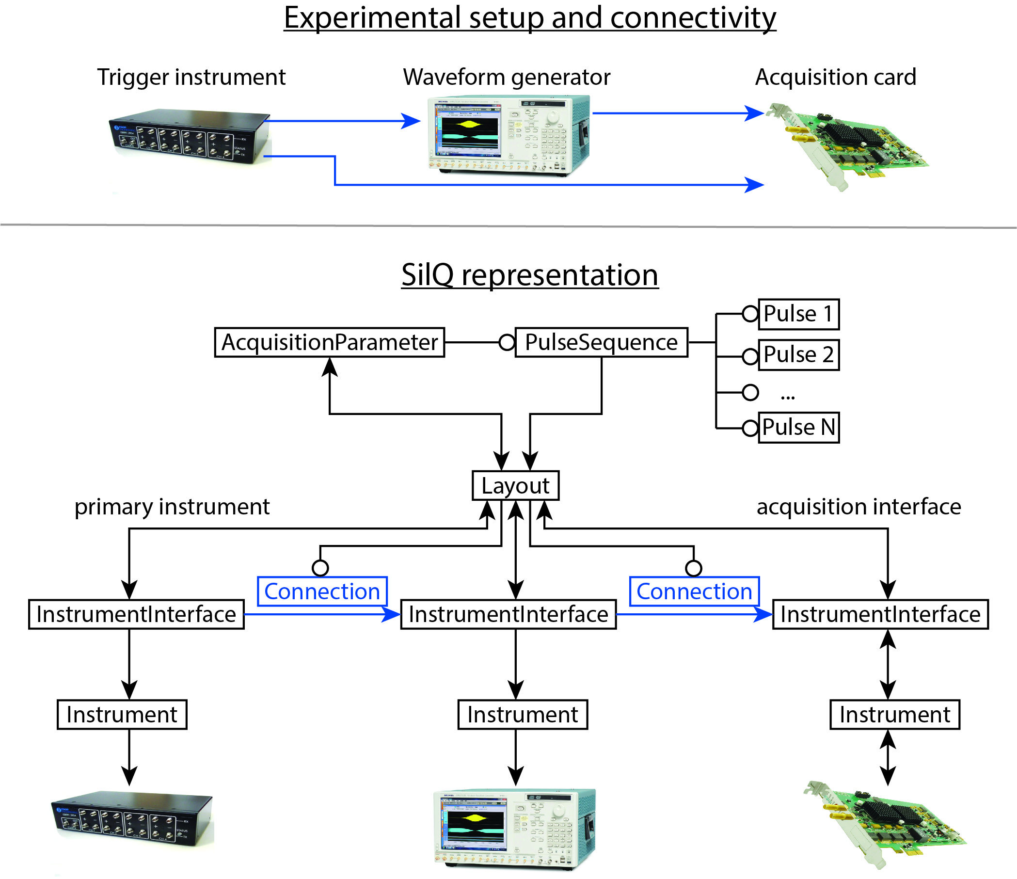
The experiment shown above is a simplified version of a typical experimental setup. It only contains three instruments, and for simplicity we ignore any sample being experimented on. A trigger instrument (left) handles the timing of the system by sending periodic triggers to the other instruments to indicate an event. The waveform generator (middle) can output waveforms (pulses). It receives triggers from the trigger instrument to indicate that it should output the next pulse. Alternatively, a trigger can indicate that it should output the entire pulse sequence and wait for the next trigger (this is usually the case for experiments requiring nanoscale precision). The waveform generator emits the pulses to the acquisition card, which is programmed to record a fixed-duration digitized signal when it receives a trigger from the trigger instrument. By programming the instruments correctly, the acquisition card can be setup to record specific pulses from the waveform generator.
Even such a simple measurement as the one described above requires many
commands to be sent to the different instruments.
In SilQ, this is handled by the Layout targeting a PulseSequence to the
particular experimental setup.
The bottom of the figure shows how the different SilQ objects interact with
one another when targeting a PulseSequence.
The arrows indicate the direction of communication, a round dot indicates
being a property of the class the line originates from.
Blue lines indicate a Connection between the
InstrumentInterfaces (there is also a connection between
the left-most and right-most interface).
Targeting a PulseSequence is actually a two-stage process.
However, stage zero is having preprogrammed all the Instruments,
InstrumentInterfaces, and Layout.
This does not mean manually sending all the commands to output the pulse
sequence, but specifying the parameters that are freely configurable,
such as the``sample rate``.
Stage 1 - Pulse distribution
The first stage is invoked by setting the Layout PulseSequence:
>>> layout.pulse_sequence = pulse_sequence
In the first step, no instruments are actually configured, but instead the
Layout passes the Pulses around to the different
InstrumentInterfaces.
These then verify that they can program their instrument to output the pulse,
and optionally request ancillary pulses from the Layout (such as trigger
pulses).
If any InstrumentInterface is not able to program its instrument to output
all the required pulses, an error is raised.
If the first does not raise any errors, then each of the InstrumentInterfaces will have its InstrumentInterface.pulse_sequence
filled with the pulses it should output.
Additionally, InstrumentInterface.input_pulse_sequence contains a list of
pulses that it receives.
All Pulses in the PulseSequence that have Pulse.acquire = True
are passed onto the acquisition InstrumentInterface.input_pulse_sequence.
This is a good moment to see if the InstrumentInterfaces have pulse sequences that actually make sense.
Note
When Layout.pulse_sequence is set to a new PulseSequence, a copy of the
PulseSequence can be stored on the computer as a python pickle with a
timestamp.
This can be useful as a logging feature, as the timestamp allows you to see
what PulseSequence was targeted at a given time.
See Storing PulseSequences for more information.
Stage 2 - Instrument setup
The second stage consists of programming the Instruments. This is invoked by calling
>>> layout.setup()
At this point the Layout signals all the InstrumentInterfaces to program their Instruments.
Each InstrumentInterface will convert its PulseSequence into
Instrument commands, and execute them.
At this stage, errors may also be raised.
This is often the case when an instrument command cannot be executed by the
instrument.
Running a pulse sequence
Once the Layout has successfully targeted a PulseSequence, the pulse
sequence can be executed on the experimental setup.
This generally happens in three steps.
Step 1 - Starting instruments
The first step consists of starting the instruments, and is called by
>>> layout.start()
The order of starting Instruments is based on their hierarchy:
instruments that need to be triggered are started
before the instrument that performs the triggering.
At the top of the chain is the primary_instrument (in this case the
triggering instrument), which is started last.
This ensures that all other instruments are awaiting a trigger and thus are
synchronized.
When the primary_instrument is started, the pulse sequence is being output
by the instruments.
Note
If the PulseSequence of any InstrumentInterface is empty, i.e. it does
not need to output pulses, it won’t be started.
Step 2 - Acquiring data
Once the pulse sequence is running, the acquisition instrument, specified by
layout.acquisition_interface, can be used to acquire a signal.
Data acquisition can be performed by calling
>>> layout.acquisition()
At this point the acquisition instrument will acquire traces and pass them
onto its InstrumentInterface.
The InstrumentInterface will then segment the traces for each of the pulses.
This way, each pulse in its input_pulse_sequence (which all have
Pulse.acquire = True) has its corresponding measured traces.
At this point, optional averaging of the traces, specified by Pulse.average,
is also performed.
When traces are acquired, more than one channel can be measured.
These channels are specified in Layout.acquisition_channels, and each channel
is given a label.
This allows the different acquisition channels to have meaningful labels (e.g.
chip output) instead of channel indices (e.g. channel_A).
The Layout attaches these labels once it receives the processed traces from
the acquisition InstrumentInterface.
Note
The number of traces is specified by
Layout.samples.Layout.start()is called if the instruments have not yet been started.
Step 3 - Stopping instruments
The final step is to stop the instruments after the acquisition is finished, and can be called by
>>> layout.stop()
This will stop the instruments according to the same hierarchy used when
starting the instruments.
This step actually happens by default at the end of an acquisition (step 2).
However, since there is overhead involved in stopping/starting instruments, it
can be ignored by calling layout.acquisition(stop=False).
Note
layout.stop() is a useful command if you want to be absolutely sure
that all instruments are not outputting anything.
It will stop all instruments, even those that aren’t involved in the
PulseSequence, and does not raise an error if instruments are already
stopped.
Summary
Although there are many steps involved in setting up and running a
PulseSequence, most of this happens under the hood.
If the InstrumentInterfaces and Layout have been
set up correctly, this whole process can be executed with just three commands:
>>> layout.pulse_sequence = pulse_sequence
>>> layout.setup()
>>> traces = layout.acquisition()
AcquisitionParameter
Performing a pulse sequence and acquiring its traces is usually only half the story; the traces often need to be analysed afterwards. While the complicated analysis should be done at a later point (potentially in an analysis notebook, initial postprocessing can usually be done straight away. Examples are measuring if a trace has a spike (blip) in current, or performing IQ demodulation of the output signal. This postprocessing is usually dependent on the type of measurement performed, and is therefore inherently linked to the pulse sequence.
The goal of the AcquisitionParameter is to combine the PulseSequence with
the corresponding postprocessing analysis, such that the user performs a
measurement, and gets the processed data straight away.
Each AcquisitionParameter has a specific PulseSequence
(AcquisitionParameter.pulse_sequence)and analysis
(AcquisitionParameter.analysis()) attached
to it.
This does not mean that the PulseSequence is fixed; its properties can
still be modified.
However, the analysis usually analyses traces of specific Pulses in
the PulseSequence, and so these pulses need to be present.
As its name suggests, an AcquisitionParameter is a
Parameter and not a ParameterNode.
The main reason is that you can use an AcquisitionParameter in a
measurement Loop as you would any other
Parameter.
The AcquisitionParameter contains the attribute names, which is a list of
things that the analysis returns.
Each of these is saved in the DataSet during a
Loop.
By default, calling AcquisitionParameter.get()
performs the following tasks:
Target its pulse sequence
Setup instruments
Start instruments
Perform acquisition
Stop instruments
Perform its analysis and return results.
The AcquisitionParameter has a rich set of options/features, for more
information see in-depth guides/AcquisitionParameter guide.
Note
The raw traces can also be saved during a measurement
Loop, see Saving traces.